강의 들으면서 중요한 것 & 알게된 것 & 느낀점 정리!
[W1] Introduction to Deep Learning
- 정형 (Structured) 데이터 & 비정형 (Unstructured) 데이터
정형 데이터: databased of data. 각각의 feature가 매우 잘 정의 됨
비정형 데이터: raw audio, image, text 등의 데이터
[W2] Logistic Regression
1. Binary Classification
: 라벨이 1 or 0으로만 구성. 예를들어 고양이 인지(1) 아닌지(0) 구분하는 문제
2. Logistic Regression
: Binary Classification을 하기 위해 활용됨.
- Output: $\hat{y}=sigmoid(W^Tx+b)$
- $W^Tx+b$ 출력을 0에서 1사이 값으로 mapping하기위해 sigmoid 사용
- $\hat{y}$ 는 x가 주어졌을 때 y=1일 확률: $\hat{y}=P(y=1|x)$
- Parameters: $W$ and $b$
3. $W$와 $b$를 학습하기 위해서 Cost function 정의
여기서는 single training example에 대한 loss function을 다음과 같이 정의한다:
$L(\hat{y}, y)=-[y \cdot log(\hat{y}) + (1-y) \cdot log(1-\hat{y})]$
이를 전체 training set에 대해, parameters ($W$ and $b$)가 얼마나 잘하고 있는지 확인하기위해 cost function $J(W, b)$ 정의:
$J(W,b)=\frac{1}{m}\sum_{i=1}^{m} L(\hat{y}^{(i)}, y^{(i)})$
4. Gradient Descent: Cost function을 최소화하는 $W$와 $b$를 찾기위한 Algorithm
최적의 W와 b를 찾기위해서, W와 b에 대한 cost function의 편미분을 계산해서 W와 b를 update. (이 부분은 그림으로 보는게 이해가 더 쉽다)
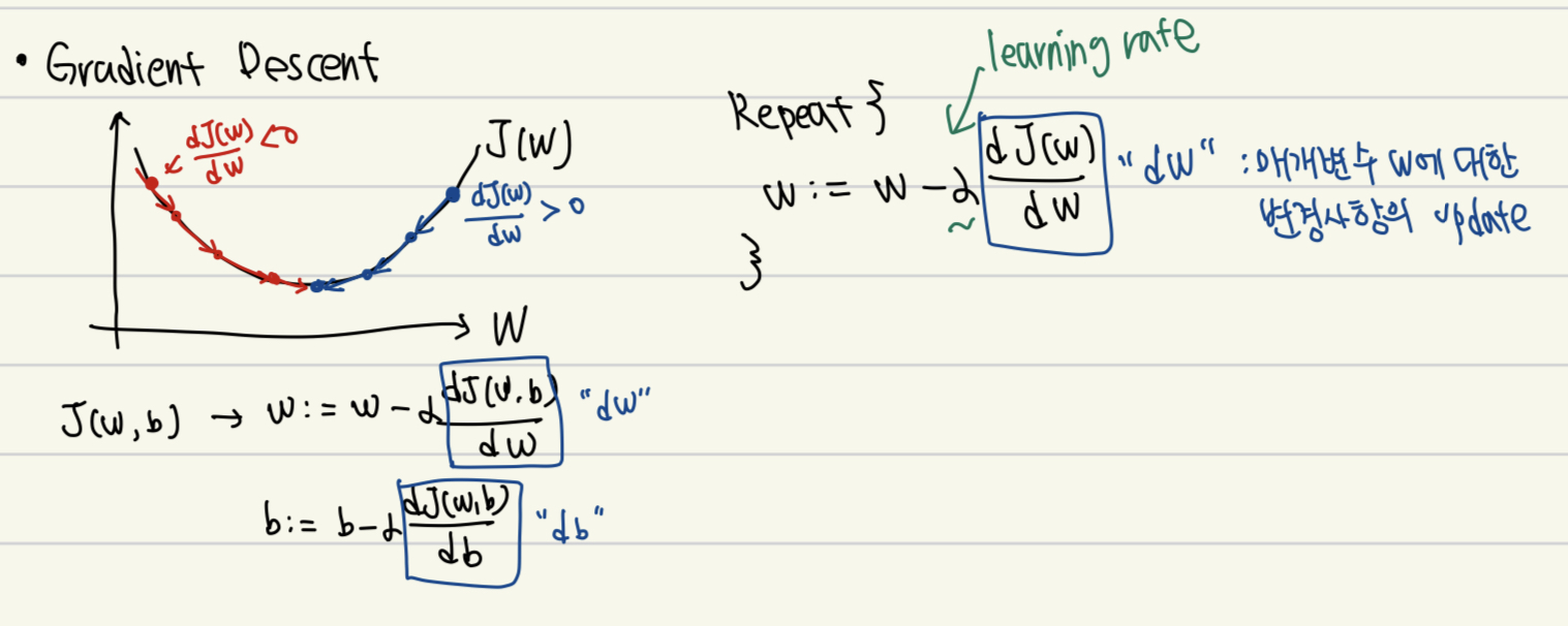
기울기가 0보다 크다면, w가 작아지는 방향으로 update 될 것이고 0보다 작다면, w가 커지는 방향으로 update 된다.
5. Logistic Regression Gradient Descent
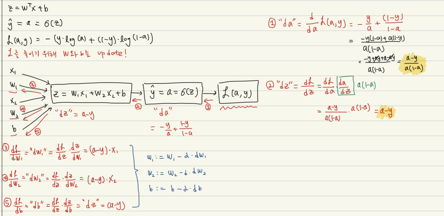
(1) Single training example에 대해서 먼저 계산해보자 (Derivatives 계산)
- $da= \frac{d}{da}L(a,y)=\frac{a-y}{a(1-a)}$
- $dz = \frac{dL}{dz} = \frac{dL}{da} \cdot \frac{da}{dz} = \frac{a-y}{a(1-a)} \cdot a(1-a) = a-y$
- $dw = \frac{dL}{dw} = \frac{dL}{dz} \cdot \frac{dz}{dw} = dz \cdot \frac{dz}{dw} = (a-y) \cdot x$
- $db=\frac{dL}{db} = \frac{dL}{dz} \cdot \frac{dz}{db} =dz \cdot \frac{dz}{db} = (a-y) \cdot 1$
(Gradient Descent: update the parameters)
$w := w - \alpha \cdot dw$ ($\alpha$: learning rate, step)
$b := b - \alpha \cdot db$
(2) m training examples에 대해 계산
: 우리의 training set에는 m개의 example이 존재한다. 전체 training set에 대해서 NN를 학습하려면 두 가지 방법이 존재한다.
- 명시적으로 for loop 활용 --> 너무 많은 시간 낭비
- Vectorization --> 두 행렬의 곱으로 수행 가능
Vectorization: column 방향으로 training example을 stack하여 하나의 큰 행렬 ($X, W, ...$)로 만든 다음 행렬 곱을 수행한다.
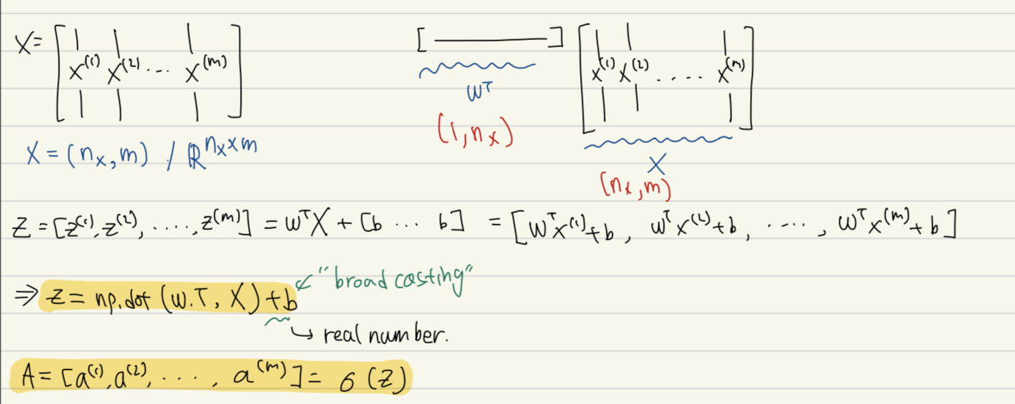
- $dZ = A-Y$
- $dW = \frac{1}{m}XdZ^{T}$
- $db = \frac{1}{m}$ np.sum($dZ$, axis=1, keepdims=1)
'ML || DL > 이론' 카테고리의 다른 글
| [Coursera] DLS_C2W1: Practical Aspects of Deep Learning (0) | 2023.09.09 |
|---|---|
| [Coursera] Neural Networks and Deep Learning 수료증 (0) | 2023.09.08 |
| [Coursera] DLS_C1W4: Deep Neural Network (DNN) (0) | 2023.09.08 |
| [Coursera] DLS_C1W3: Shallow Neural Networks (0) | 2023.09.06 |
| [DeepMind x UCL] Lecture 1. Intro to Machine Learning & AI (0) | 2021.01.07 |